06 Nov The Hidden Role of AI in IoT Systems (That No One Talks About)
How edge intelligence, machine learning, and continuous feedback are redefining what it means to build a “smart” device.
AI in IoT systems is no longer about connecting devices. It’s about closing the loop between perception, decision, and action. Most engineers still see IoT as a linear pipeline. They think data goes up, insights come down. But the truth is, every intelligent system runs on a hidden feedback loop. This hidden feedback loop is the one that senses, infers, acts, and learns in real time. This loop is what separates “connected” from conscious, and it’s quietly reshaping how modern embedded systems, industrial controllers, and edge devices evolve after deployment.
1. The Illusion of “Smart” Devices
Every product today claims to be smart, from thermostats that “learn” your habits to industrial sensors that “predict” downtime. The marketing sounds intelligent. But peel back the firmware, and most of these so-called intelligent devices are just reactive circuits with cloud connectivity.
AI in IoT systems isn’t about adding buzzwords to dashboards. It’s about embedding reasoning into the physical world. True intelligence doesn’t stop at data collection: it forms a loop. The sensor detects a change, the system interprets it, executes a response, observes the result, and refines itself over time. That’s not a one-way data pipeline; that’s a closed-loop learning architecture.
The problem is that most systems today never complete that loop. Data flows upward to analytics platforms, models are trained once, and devices continue operating with static logic. They sense, maybe even infer, but they rarely learn. The gap between insight and adaptation is where most IoT projects stall, and where the next generation of engineering breakthroughs is happening.
We’ve at AMSIoT learned that a system doesn’t become “smart” by training a neural network once. It becomes intelligent when that model is anchored to feedback, constantly tuned by real-world inputs. That’s the difference between devices that simply monitor conditions and systems that self-correct under changing environments: from vibration sensors in factories that adjust thresholds autonomously, to energy meters that recalibrate based on behavioral drift.
The illusion of smartness ends the moment an IoT device stops learning. And the engineers who understand this hidden loop are the ones building the future of adaptive systems.
2. The Hidden Mechanism Beneath Every IoT System
If you strip an IoT architecture down to its essence, you’ll find one universal structure: a loop. Not a network topology or data flow chart, but a biological-like feedback cycle that connects sensing, decision, and adaptation. Every truly intelligent system, whether it’s a smart grid, an autonomous vehicle, or a temperature controller: revolves around this continuous process.
At AMSIoT, we call it the AI Feedback Loop. It’s what gives static devices dynamic intelligence: the ability to react, improve, and eventually predict.
2.1 The Four Phases of Intelligence
Every adaptive IoT system runs through four technical stages, each reinforcing the other:
Sense: Capture what’s happening.
Infer: Decide what it means.
Act: Respond in real time.
Learn: Improve with experience.
It sounds simple, but the challenge lies in how engineers implement these transitions. Let’s break down what happens between the arrows.
From Sense to Infer: Turning Signals into Meaning
Raw data doesn’t equal understanding. Temperature sensors, accelerometers, and pressure transducers might generate gigabytes of readings. But without edge AI models, they’re just noise. The real engineering challenge is converting analog reality into a digital context. This includes filtering noise, extracting features, and classifying behavior in milliseconds.
This is where machine learning in IoT comes alive. A trained model at the edge identifies that a vibration spike isn’t random; it’s an early sign of mechanical imbalance. The faster this inference happens, the closer your system moves toward autonomy and away from manual monitoring.
From Infer to Act: Closing the Physical Loop
Most systems stop here: they detect anomalies but send them to the cloud, waiting for human intervention. That latency kills adaptability.
The next phase, action, is where intelligence becomes tangible. Microcontrollers trigger control relays, servo motors adjust, or power regulators shift states: all within milliseconds.
When properly engineered, these reactions form a control feedback layer: responsive yet safe. The cloud still exists, but not as a decision-maker; it becomes a teacher, logging results and preparing the next model update.
2.2 Where Most Systems Fail
Here’s the catch: almost 80% of deployed IoT systems never reach the Learn phase. They collect terabytes but rarely loop that data back into model refinement. The missing piece isn’t technology, it’s design philosophy.
Most engineers still think in linear architectures: Sensor → Gateway → Cloud → Dashboard. But intelligent systems demand cyclic architectures, where the output of today becomes the input for tomorrow.
That’s the hidden AI loop: a closed, continuous system where sensing, inference, action, and learning feed each other indefinitely. It’s not about building smarter dashboards; it’s about engineering self-correcting ecosystems.
3. Sense: The Foundation of Perception
Every intelligent loop starts with perception. In AI in IoT systems, the Sense phase defines the entire ceiling of intelligence: if the signal is noisy, biased, or delayed, no algorithm downstream can save it. Smart systems aren’t born in Python notebooks; they’re born at the ADC pin.
3.1 From Physics to Data
Sensors are the nervous system of any IoT node. They convert physical phenomena vibration, temperature, voltage, torque into measurable electrical signals. But the engineering precision in this conversion determines how well AI models can learn patterns later.
A simple accelerometer, for example, can deliver anywhere between 8-bit and 20-bit resolution. For a predictive-maintenance model, that difference decides whether the network detects a bearing defect two days early or two seconds before failure.
Hence, AMSIoT engineers design from the signal chain backward:
- Analog front-end filtering (RC or active) eliminates out-of-band noise.
- Oversampling + decimation improves SNR without overloading bandwidth.
- Synchronous sampling across channels ensures phase integrity for multi-sensor fusion.
Only then does “data” become trustworthy enough for AI inference.
3.2 Embedded Intelligence at the Edge From Sensor Stream to Real-Time Decision
The Infer stage begins where signal conditioning ends. After the analog world has been digitized and pre-filtered, intelligence must occur as close to the sensor as possible to minimize latency and bandwidth. In modern AI in IoT systems, this is achieved through edge inference, where a microcontroller or SoC executes a compact ML model directly on the device.
Architecture Overview
A typical AMSIoT edge-AI node integrates the following stack:
| Layer | Function | Typical Hardware/Software |
| Sensor Interface | SPI/I²C/ADC acquisition with DMA buffering | STM32 ADC + DMA, ESP32 ADC DMA |
| Signal Conditioning | FIR/IIR or digital notch filters implemented in ISR or DMA post-processing | CMSIS-DSP, ESP- DSP |
| Feature Extraction | Real-time windowing (e.g., 256–512 samples), FFT/PSD, energy ratios, statistical descriptors | Arm CMSIS-DSP, MicroMLGen |
| Model Execution | Quantized ML inference (int8 or uint8) with fixed- point math | TensorFlow Lite Micro, Edge Impulse SDK |
| Decision & Control | Output thresholding, hysteresis, GPIO/CAN/MQTT trigger | FreeRTOS tasks, CANOpen stack |
Each layer executes within a deterministic control loop, typically 20 – 100 ms per inference cycle. Thus, this allows the closed-loop control for mechanical or process-driven systems.
Data Pipeline Details
Windowing & Pre-processing
Sensor streams are segmented into sliding windows using ring buffers. Let’s say a 1 kHz accelerometer feed with 256-sample windows provides 3.9 inferences/s with 75 % overlap. Real-time filtering (moving-average, band-pass) removes alias components before feature computation.
Feature Computation
Common feature sets:
- Time-domain: mean, RMS, skewness, kurtosis.
- Frequency-domain: FFT magnitude bins, spectral centroid, bandwidth.
- Statistical/entropy: Shannon entropy, crest factor. These features form a fixed-length vector f ∈ ℝⁿ (typically 8–64 elements).
Model Inference
Models are trained offline (Python/TensorFlow or scikit-learn) and converted using TensorFlow Lite Converter with post-training quantization. On-device, the interpreter executes integer arithmetic on MCU DSP cores.
Typical footprint:
- Model size: < 150 KB
- SRAM: < 256 KB
- Latency: < 30 ms @ 80 MHz AMSIoT often employs:
- Decision Tree / Random Forest: low-power classification of discrete states.1-D CNN: frequency-pattern detection for vibration or acoustic data.
- LSTM / GRU: temporal prediction for energy or usage forecasting.
Decision Logic
The output vector y = [ p₀, p₁, … , p◻ ] is post-processed by confidence gating and hysteresis to prevent oscillation. Threshold crossings trigger hardware actions via ISR or RTOS queues, such as reducing motor duty-cycle, activating a relay, or publishing a JSON packet through MQTT.
Optimization Techniques
- Quantization-aware training (QAT): preserves accuracy after int8 conversion.
- Pruning / weight-sharing: reduces Flash usage by 30–50 %.
- CMSIS-NN kernels: leverage SIMD on Cortex-M cores for 2–3× speed-up.
- Duty-cycling inference: alternate sensing and sleep phases for sub-milliamp power budgets.
- On-device buffering & circular DMA: prevents ISR blocking, sustaining deterministic timing.
System-Level Integration
Edge-AI nodes typically publish both classified states and confidence metrics via MQTT/Modbus TCP. At AMSIoT, gateway firmware aggregates these metrics for fleet-level learning. The cloud retrains global models while each node remains autonomous. This hybrid architecture preserves low-latency response while enabling long-term improvement a practical embodiment of the Sense → Infer → Act → Learn loop.
3.3 Calibration and Drift Handling
Even perfect sensors age, and data drift is the silent killer of long-term reliability. AMSIoT’s systems employ auto-calibration routines that periodically benchmark baseline values, then compensate offsets through firmware. On the analytical side, statistical control charts or online normalization adjust feature scaling dynamically, maintaining inference accuracy despite hardware or environmental shifts.
To further explain this concept: A temperature node deployed in a humid plant may see sensor offset drift by ±2 °C over 90 days. Without periodic recalibration, the ML model’s threshold confidence collapses. Closing the loop between firmware calibration ↔ model retraining ensures the Sense layer remains a reliable foundation.
3.4 Why It Matters
In adaptive IoT design, perception errors cascade. A mis-timed vibration sample leads to a misclassified anomaly, which triggers a false shutdown, which costs production hours. That’s why the “smartness” of AI in IoT systems doesn’t start in the algorithm it starts in the analog domain, where real-world fidelity meets digital intelligence.
4. Infer is Where AI Actually Thinks
After the sensing layer has translated physics into clean, calibrated data, the Infer phase determines whether that information becomes intelligence or remains telemetry. In AI in IoT systems, this is the layer where algorithms start behaving like reasoning agents rather than loggers.
4.1 Inference as a Real-Time Control Process
At this stage, every microsecond counts. An inference pipeline in an AMSIoT-grade node typically executes inside a deterministic control loop (RTOS task or ISR context). Each cycle performs:
Acquire + Pre-process: Pull buffered window from DMA, normalize, filter.
Infer: Execute the compiled ML model (decision tree / 1-D CNN / LSTM) using fixed-point math on the MCU’s DSP core.
Decide: Map output probabilities to operational states.
Dispatch: Send control flags to actuators or upstream gateways.
The loop period must be shorter than the process time constant (usually ≤ 50 ms for mechanical systems). Missing that deadline turns “AI” into latency. That’s why AMSIoT designs its embedded models with constant-time execution and predictable memory footprints a requirement that cloud engineers often underestimate.
4.2 Model Types and Deployment Topologies
Different tasks demand different model geometries:
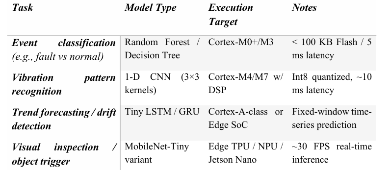
All models undergo post-training quantization and layer fusion to fit embedded constraints without losing more than 2–3 % accuracy.
Deployment patterns vary:
- On-Device Inference: Low latency, privacy-preserving, ideal for critical loops.
- Edge-Gateway Inference: Aggregates multiple sensor nodes; mid-latency (~100 ms); allows heavier models.
- Hybrid Inference: Local classification + cloud re-validation for drift tracking and retraining.
4.3 Confidence Gating and Decision Logic
Intelligence is useless without stability. AMSIoT implements confidence-gated state transitions:
𝑆𝑖,𝑃𝑖 > 𝜏ℎ
State(t+1)= 𝑆𝑡, 𝜏𝑙 < 𝑃𝑖 < 𝜏ℎ
𝑆𝑗,𝑃𝑗 > 𝜏ℎ
where 𝑃𝑖is the probability of state i, 𝜏ℎand 𝜏𝑙are high/low hysteresis thresholds. This prevents oscillations in actuator control when inference outputs fluctuate around a decision boundary. Each decision event is time-stamped and logged to flash or buffer memory, forming a ground-truth trace later used for model retraining (the bridge to the Learn phase).
4.4 Performance and Diagnostics
Key runtime diagnostics include:
- Inference Latency: measured via hardware timers must stay < 5 % of lthe loop period.
- CPU Load & Heap Usage: monitored to detect memory fragmentation; critical for 24/7 systems.
- Confidence Entropy: 𝐻 = ―∑𝑝𝑖log 𝑝𝑖; rising entropy signals concept drift.
- Thermal Envelope: especially in sealed industrial enclosures, CPU overheating reduces clock frequency and misses deadlines.
AMSIoT’s runtime profiler collects these metrics over MQTT/Modbus, streaming them to a cloud dashboard for predictive diagnostics on the AI pipeline itself meta-monitoring of intelligence.
4.5 From Inference to Action
When the inference engine reaches a high-confidence decision, the Act layer executes: adjusting PWM, switching contactors, publishing commands, or updating a process variable. Crucially, the loop doesn’t end here. The outcome of every actuation (success/overshoot/error) is logged and labeled automatically, providing the raw data for continuous learning.
This tight coupling between inference and control is what transforms static automation into
adaptive intelligence a living system that evolves in production.
5. Closing the Loop From Data to Intelligence
5.1 Where Data Ends and Intelligence Begins
The transition from raw data to meaningful action is not a step; it’s a convergence. When the Sense layer captures clean, synchronized signals and the Infer layer interprets them with deterministic latency, the system reaches a threshold where data becomes behavior. This convergence marks the moment IoT crosses from “monitoring” into “thinking.”
At AMSIoT, this boundary is treated as a design checkpoint: the device must demonstrate that it not only measures accurately but also understands causality between what it senses and what it predicts. That understanding is the signature of a functioning AI in IoT system. Everything that follows the actual execution of actions and the assimilation of their outcomes will complete the cycle that turns smart devices into living systems.